Comment Analysis of the Mathematica StackExchange
For this post, I’m going to use a bunch of data I mined a few posts back to do a basic analysis of the comments on a forum like StackExchange. As per usual, I’m going to focus on the Mathematica StackExchange, as that is in some sense my “home” community on the network.
I’m going to make all of this data publically accessible via the Wolfram Cloud . It will live here:
KeyChainConnect["DatasetsAccount"]

(*Out:*)

"b3m2a1.datasets@gmail.com"

CloudObject["stack_exchange_data"][[1]]

(*Out:*)

"https://www.wolframcloud.com/objects/b3m2a1.datasets/stack_exchange_data"
Obtaining the Data
Finding a set of commenters
To start off, let’s import the cached version of my Mathematica user list:
mUsers =
   CloudImport["stack_exchange_data/communities/mmaUsers.mx"];
Let’s then look at the different metrics we have to do analyses on:
DeleteDuplicates[Flatten[Normal@Keys[mUsers]]] // Sort

(*Out:*)

{"accept_rate", "account_id", "age", "badge_counts", "creation_date",
"display_name", "is_employee", "last_access_date",
"last_modified_date", "link", "location", "profile_image",
"reputation", "reputation_change_day", "reputation_change_month",
"reputation_change_quarter", "reputation_change_week",
"reputation_change_year", "timed_penalty_date", "user_id",
"user_type", "website_url"}
There are lots of things we could roll with here, but I think the two *most generally useful* ones will be the "age" and "location" parameters. Since I looked at ages last time, lets look at them again.
First we’ll correlate age with IDs:
idAges =
   DeleteMissing@Dataset@Association@Flatten@Normal[
         mUsers[All, #["user_id"] -> #["age"] &]];
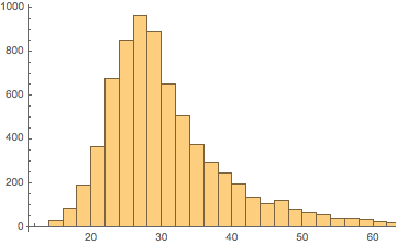
Then histogram out our ages again, just to recall what they looked like:
Histogram[Values[idAges]]

(*Out:*)
Next we’ll see how we can gather user comments:
$so = ServiceConnect["StackExchange"]

(*Out:*)

The request for this will be the "UserComments" request:
htmlImp[ds_] :=

  ImportString[StringRiffle[Normal[ds[All, "body"]], "<br/><br/>"],
   "HTML"];
htmlImp@$so[
   "UserComments",
   "id" -> Keys[idAges][[1]], "site" -> "mathematica",
   "filter" -> "withbody",
   "pagesize" -> "5"
   ]
-----------Out-----------
Thanks for the info, that's good to know.

Let us continue this discussion in chat .

I will look into that, but you are the first one to report this problem. Are you sure it is not on your side (your reader)? I have not touched the pdf pretty much since I uploaded it back in 2009.

@AliHashmi Thanks. But it's been here for quite a while.

@b3m2a1It has been cross-platform since V10, if memory serves. With the caveats mentioned by Szabolcs.
If we look at how long one of these requests at full size takes:
htmlImp@$so[
     "UserComments",
     "id" -> Keys[idAges][[1]],
     "site" -> "mathematica",
     "filter" -> "withbody",
     "pagesize" -> "100"
     ] // AbsoluteTiming // First

(*Out:*)

1.46333
We find that we definitely don’t want to do this for the full 7156 users. Given that I probably only am wiling to wait 5 minutes for this data to come in and have 8 cores to distribute over, let’s figure out how large a sample we can use:
timing =
   htmlImp@$so[
        "UserComments",
        "id" -> Keys[idAges][[1]],
        "site" -> "mathematica",
        "filter" -> "withbody",
        "pagesize" -> "100"
        ] // AbsoluteTiming // First;
Quantity[5*8, "Minutes"]/Quantity[timing, "Seconds"]

(*Out:*)

1432.56
So let’s take like 1500 users, where we try to get pretty even sampling over ages. To do this, we can first try to fit our data to an ExtremeValueDistribution :
oldDist =
  EstimatedDistribution[Normal@Values@idAges,
  ExtremeValueDistribution[α, β]]

(*Out:*)

ExtremeValueDistribution[26.8155, 6.90588]
And then we’ll weight by the reciprocal of this:
newIdAges =
   RandomSample[
     Values[#] -> Keys[#] &@
       Normal[Map[Evaluate[1/PDF[oldDist, #]] &, idAges]],
     1500
     ];
Then just to see how well we did:
SmoothHistogram[
  {
    Lookup[Normal@idAges, newIdAges],
    Normal@Values[idAges]
    },
  PlotRange -> All
  ]

(*Out:*)
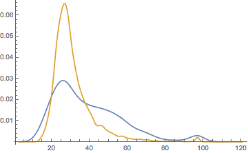
We find that this did help smooth the distribution. But we might want to try to do a bit better. For that we could use a real SmoothKernelDistribution .
oldDist =
   SmoothKernelDistribution[Normal@Values@idAges];
newIds =
   RandomSample[
     Values[#] -> Keys[#] &@
       Normal[Map[Evaluate[1/PDF[oldDist, #]] &, idAges]],
     1500
     ];
SmoothHistogram[
  {
    Lookup[Normal@idAges, newIds],
    Normal@Values[idAges]
    },
  PlotRange -> All
  ]

(*Out:*)
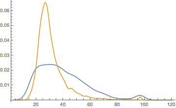
Which seems to have worked much better.
Extracting the comments:
With this in mind, we’re almost set actually mine this data. First let’s just do some quick checks that our users really have comments to their names:
AbsoluteTiming[
   comms =
     AssociationMap[
       $so[
          "UserComments",
          "id" -> #,
          "site" -> "mathematica",
          "filter" -> "withbody",
          "pagesize" -> "1"
          ] &,
       newIds
       ]
   ] // First

(*Out:*)

131.471

Select[comms, Length[#] > 0 &] // Length

(*Out:*)

375
So we’re down to 375 users. Which is, I suppose, not terrible, but we’ll at least try to pad it back up a bit:
newIds2 =
   RandomSample[
     Values[#] -> Keys[#] &@
       Normal@
         Map[
           Evaluate[1/PDF[oldDist, #]] &,
           KeyTake[idAges,
             Complement[Keys@idAges, newIds]
             ]
           ],
     1500
     ];
And then once more we’ll prune like this:
AbsoluteTiming[
   comms2 =
     AssociationMap[
       $so[
          "UserComments",
          "id" -> #,
          "site" -> "mathematica",
          "filter" -> "withbody",
          "pagesize" -> "1"
          ] &,
       newIds2
       ]
   ] // First

(*Out:*)

129.244

Select[comms2, Length[#] > 0 &] // Length

(*Out:*)

348
So between the two of these we have ~700 users. Still not many, but enough to start with.
Finally, we’ll get to mining the comments:
AbsoluteTiming[
   idComments =
      AssociationMap[
        $so[
            "QueryIterate",
            "Request" -> "UserComments",
            "id" -> #,
            "site" -> "mathematica",
            "filter" -> "withbody",
            "MaxIterations" -> 10
            ] &,
        Keys@Join[
           Select[comms, Length[#] > 0 &],
           Select[comms2, Length[#] > 0 &]
           ]
        ];
   ][[1]]

(*Out:*)

307.98
And then we’ll dump these onto the cloud:
CloudExport[idComments, "MX",
"stack_exchange_data/comments/mmaComments.mx",
  Permissions -> "Public"
  ]

(*Out:*)

CloudObject["https://www.wolframcloud.com/objects/b3m2a1.datasets/stack_exchange_data/comments/mmaComments.mx"]
Distributions in Mathematica StackExchange comments
User comment counts
Let’s just start by view in the distribution of comment numbers by user:
SmoothHistogram[
  idComments // Map[Length] // Values,
  PlotRange -> All
  ]

(*Out:*)
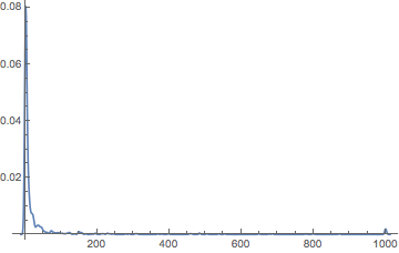
Which, somewhat unsurprisingly, shows a major peak around no comments and a minor peak at more-comments-than-I-imported. Of course, it is these comments by a small fraction of the site’s users that will tend to dominate this discussion, and they are simply so much more numerous (and generally longer).
Comment lengths
We can also break these apart by length:
imppedComments =
   StringSplit[htmlImp@Apply[Join, Values[idComments]], "\n\n"];
And given that that took a little to run, we can also dump this into the cloud:
CloudExport[imppedComments, "MX",
"stack_exchange_data/comments/mmaSplitComments.mx",
  Permissions -> "Public"
  ]

(*Out:*)

CloudObject["https://www.wolframcloud.com/objects/b3m2a1.datasets/stack_exchange_data/comments/mmaSplitComments.mx"]
Then we can look at average comment length:
comLens = StringLength /@ imppedComments;
SmoothHistogram[comLens]

(*Out:*)
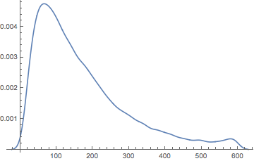
A few features stand out in this. The first is that we likely have two to three distributions hidden in here, which we can try to model as a MixtureDistribution of GammaDistributions and NormalDistributions .
We’ll start by letting Mathematica provide a guess and comparing that to our observed distribution:
comLenDist =
  FindDistribution[comLens,
    TargetFunctions -> {NormalDistribution, GammaDistribution},
    PerformanceGoal -> "Quality"
    ]
Show[
  SmoothHistogram[comLens],
  Plot[PDF[comLenDist, x],
    {x, 0, 650},
    PlotStyle -> ColorData[97][2]
    ],
  PlotRange -> All
  ]

(*Out:*)

MixtureDistribution[{0.83119,
  0.16881}, {GammaDistribution[2.37578, 56.2346],
  NormalDistribution[350.011, 133.508]}]

(*Out:*)
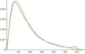
Which is, overall, a pretty good guess. But notably it misses that little hump up around 590 that I would argue is meaningful. So we’ll use this form as a base and add another distribution:
comLenDist =
  EstimatedDistribution[
    comLens,
    MixtureDistribution[
      {big, mid, little},
      {
        GammaDistribution[α, β],
        NormalDistribution[μ, σ],
        NormalDistribution[μs, σs]
        }
      ],
    MixtureDistribution[
      {0.83, 0.17, .05},
      {
        GammaDistribution[2.73, 56.23],
        NormalDistribution[350.01, 133.51],
        NormalDistribution[590, 10]
        }
      ],
    AccuracyGoal -> 20
    ]

(*Out:*)

MixtureDistribution[{0.823455, 0.158972,
  0.017573}, {GammaDistribution[2.4218, 53.6177],
  NormalDistribution[331.916, 108.543],
  NormalDistribution[571.785, 19.2683]}]

Show[
  SmoothHistogram[comLens],
  Plot[
    PDF[comLenDist, x],
    {x, 0, 650},
    PlotStyle ->
     	ColorData[97][2],
    PlotRange -> All
    ],
  PlotRange -> All
  ]

(*Out:*)
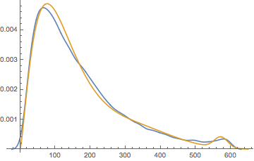
We’ve lost some goodness of fit, but have recovered one of the obvious features of the distribution, so we’ll call that a win for now.
What’s interesting about this is the form. We can view this as its component distributions:
Plot[
  Evaluate@
    Prepend[
      MapThread[#*PDF[#2, x] &, List @@ comLenDist],
      PDF[comLenDist, x]
      ],
  {x, 0, 650},
  PlotRange -> All
  ]

(*Out:*)
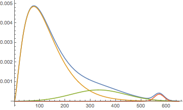
The feature up above 500 can be easily assigned to the reasonably common case where the allotted number of characters is insufficient. Often this even causes wrapping over into further comments.
The case of the primary peak around 100 is again reasonable, if perhaps on the high side. Seeing as this sentence is ~100 characters, we can conclude that most comments are about a sentence long. If this seems high compared to general experience this may illustrate how little that is:
StringRiffle[
  RandomSample[
    MinimalBy[
      Select[imppedComments, StringLength[#] == 100 &],
      StringLength
      ],
    5
    ],
  "\n\n"
  ]
-----------Out-----------
You'll probably have to write a webscraper. At least according to stackoverflow.com/q/5991756/421225

@user11946 I suggest you take a look at the tutorial here: reference.wolfram.com/language/tutorial/…

(# - 2)^2 (# + .5)^2 - 625/256 &[x], it seems that not all the roots can be found for this function.

There seems to be a bug. I get 5 for HenrikfindIndices[{0.1,0.2,0.3,0.6,0.8}, .7] and I expected 4 .

Please provide definitions for borderGCVector and linkGCVector . Your code doesn't run without them.
On the other hand, even the absolute longest comments aren’t that much text. Here’re a few of them:
StringRiffle[
  RandomSample[
    TakeLargestBy[imppedComments, StringLength, 10],
    2
    ],
  "\n\n"
  ]
-----------Out-----------
@Pickett And when I saw it, I thought my world was about to change :-), but after discussing it with some more "knowledgeable people", although it was clear that the scope of these products was not yet very clear (or at least, to them), they all said that this would most likely be products to be integrated/used by editors of other products (that is medium to large scale businesses), and not really by individual users on a one case scenario... (it would be something like special licensing schemes, etc). But this was some time ago and probably the image is more clear now, and things have changed

Dear Yode, your approach in "treating" the image is very similar to the many attempts I made, before posting this question. Nonetheless, you were very successful at getting the lines over the sugarcane. The fact that there some misses is not very important, because one can always extrapolate the missing lines by looking at the most frequent distance between two lines (in a histogram). However, you approach will not work with a curved path, because of the function ImageLines, which only yields straight lines. Nonetheless, I am certain that your method will help me to improve on mine. Thank you.
The mushy middle Gaussian is an interesting case where there’s just such a broad distribution of these random comment lengths. Looking at these isn’t particularly interesting, so we’ll leave them out.
Mathematica StackExchange comment content
Word clouds and word frequencies
Finally we can start to play with some fun stuff. To start, let’s just make a word cloud of all of this stuff:
comString = StringRiffle[imppedComments];
WordCloud[comString]

(*Out:*)

Unfortunately these aren’t terribly interesting. We could try removing some of these rather boring terms, but there’s no real reason to expect that this will dredge up anything fascinating.
We do see a few fun things, though, particularly in the prominence of single letters and numbers, like x , y , 1 , 2 , etc.
These show that this is math driven site (unsurprisingly).
So let’s move to something more quantitative. First we’ll get the words and bin them by usage:
comWords =
   TextCases[DeleteStopwords@comString, "Word"];
comCounts =
   Counts[ToLowerCase@comWords];
Again I’ll dump these into the cloud, as they are computationally expensive:
CloudExport[comCounts, "MX",
"stack_exchange_data/comments/mmaWordCounts.mx",
  Permissions -> "Public"
  ]

(*Out:*)

CloudObject["https://www.wolframcloud.com/objects/b3m2a1.datasets/stack_exchange_data/comments/mmaWordCounts.mx"]
Next we’ll take the word frequencies over these words:
wordFreqs =
   AssociationThread[
     Keys[comCounts],
     Rescale[1. Values[comCounts]]
     ];
TakeSmallest[wordFreqs, 10]

(*Out:*)

<|"whenevent[{s[1][t" -> 0., "v.11.0.1" -> 0., "249/250" -> 0.,
 "10.13" -> 0., "10.13.2" -> 0., "floor[log[10" -> 0., "2x+y" -> 0.,
 "@louisb" -> 0., "pureunities" -> 0., "x^2+y" -> 0.|>
And we see from this that these aren’t really even words. So we’ll just drop them.
wordFreqs2 =
   Select[wordFreqs, GreaterThan[.0005]];
TakeSmallest[wordFreqs2, 10]
TakeLargest[wordFreqs2, 10]

(*Out:*)

<|"mma8" -> 0.000542446, "responsive" -> 0.000542446,
 "nasserm.abbasi" -> 0.000542446, "10.10.4" -> 0.000542446,
 "ummm" -> 0.000542446, "biases" -> 0.000542446,
 "sensor" -> 0.000542446, "3.4" -> 0.000542446,
 "underdetermined" -> 0.000542446, "k3" -> 0.000542446|>

(*Out:*)

<|"question" -> 1., "answer" -> 0.941416, "code" -> 0.880662,
 "use" -> 0.803092, "1" -> 0.763765, "just" -> 0.725522,
 "mathematica" -> 0.72498, "thanks" -> 0.718742, "like" -> 0.670464,
 "function" -> 0.597776|>
These, on the other hand, are largely boring. But lets compare these frequencies to the standard WordFrequencyData to get a sense of what words might be abnormally present:
wordFreqsReal =
   WordFrequencyData[
     Keys@TakeLargest[wordFreqs2, 500]
     ];
TakeSmallest[wordFreqsReal, 15]

(*Out:*)

<|"j.m." -> 5.33713*10^-9, "mma" -> 1.52723*10^-8,
 "mathematica" -> 2.4267*10^-8, "workaround" -> 3.91462*10^-8,
 "wolfram" -> 4.27572*10^-8, "mac" -> 1.81982*10^-7,
 "pdf" -> 2.23877*10^-7, "ok" -> 4.88281*10^-7,
 "formatted" -> 6.09125*10^-7, "+1" -> 9.20242*10^-7,
 "bug" -> 1.23268*10^-6, "plotting" -> 1.63899*10^-6,
 "simplify" -> 1.77491*10^-6, "kernel" -> 1.87406*10^-6,
 "notebook" -> 1.89268*10^-6|>
This is vaguely interesting, as we see a number of Mathematica specific terms ( "workaround" , "formatted" ) show up with very low frequency. But even more interesting is that "j.m" which is a reference to a user. We’ll handle that a bit later.
For now, we’ll go back to the case at hand. We’ll take our wordFreqs2 and divide these out by out wordFreqsReal :
Take[
  wordFreqsNormmed =
    ReverseSort[TakeLargest[wordFreqs2, 500]/wordFreqsReal],
  10]

(*Out:*)

<|"mr.wizard" -> 0.127204/Missing["NotAvailable"],
 "@szabolcs" -> 0.102251/Missing["NotAvailable"],
 "{x," -> 0.0979116/Missing["NotAvailable"],
 "@kuba" -> 0.0810957/Missing["NotAvailable"],
 "{1," -> 0.0550583/Missing["NotAvailable"],
 "plotrange" -> 0.0474641/Missing["NotAvailable"],
 "@belisarius" -> 0.0466504/Missing["NotAvailable"],
 "ndsolve" -> 0.0450231/Missing["NotAvailable"],
 "@michaele2" -> 0.0450231/Missing["NotAvailable"],
 "{0," -> 0.0436669/Missing["NotAvailable"]|>
And we see two things. One, when we look at user names we’ll have to account for @ mentions. Two, there are interesting terms like "ndsolve" that simply never come up outside of this context. There are fewer of these than there are junk terms like "{0" those, so we’ll just delete all of these.
Take[Select[wordFreqsNormmed, NumberQ], 5]

(*Out:*)

<|"mathematica" -> 2.98751*10^7, "j.m." -> 1.64651*10^7,
 "mma" -> 1.22715*10^7, "wolfram" -> 2.28994*10^6,
 "workaround" -> 997700.|>
And thus things like "mathematica" explode. So we’ll drop anything with size greater than <p>10</p>6 .
Take[
  wordFreqsNorm2 =
    Select[wordFreqsNormmed, LessThan[10^6]],
  5
  ]

(*Out:*)

<|"workaround" -> 997700., "ok" -> 228296., "mac" -> 220576.,
 "pdf" -> 216856., "+1" -> 213385.|>
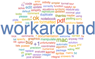
And we start to see some fun things. Particularly the prominence of the word "workaround" . This could reflect the fact that many questions on the site do seem to be about workarounds for various not-entirely-there pieces of core functionality.
But let’s word-cloud these out (dropping "workaround" as it is another outlier)
(*Out:*)
WordCloud[Rest@wordFreqsNorm2]

(*Out:*)
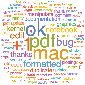
We see that "+1" is very popular relative to standard word frequency, unsurprisingly. And "workaround" gets paired with the word "bug"
Comment mentions vs. reputation
We could, in fact, extract *all* of the users whose names appear in wordFreqs2 :
userNames =
   StringDelete[
     ToLowerCase@Normal@
        Reverse@mUsers[SortBy["reputation"], "display_name"],
     Whitespace
     ];
KeyTake[wordFreqs, Take[userNames, 10]]

(*Out:*)

<|"mr.wizard" -> 0.127204, "szabolcs" -> 0.0127475,
 "michaele2" -> 0.00081367, "kglr" -> 0.00162734,
 "dr.belisarius" -> 0.00298346, "kuba" -> 0.0105777,
 "jens" -> 0.00542446, "j.m." -> 0.0878763, "halirutan" -> 0.0035259|>
And since the userNames are in reverse-reputation order this provides an interesting connection between reputation and comment mentions. Given that the API also provides a "UserMentions" request we could check this more directly, but for now we’ll use this as our proxy.
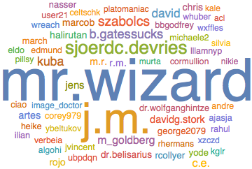
We can do a raw word cloud of the 100 highest-rep users:
WordCloud@KeyTake[wordFreqs, Take[userNames, 100]]

(*Out:*)
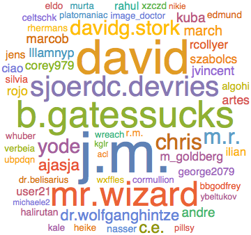
Or we can normalize these by reputation:
userNameReps =
   KeyTake[
     Association@Normal@
        mUsers[
          SortBy["reputation"],

      StringDelete[ToLowerCase@#["display_name"], Whitespace] -> #[
         "reputation"] &
          ],
     Keys@KeyTake[wordFreqs, Take[userNames, 100]]
     ];
WordCloud[
  KeyTake[wordFreqs, Keys[userNameReps]]/
    userNameReps
  ]

(*Out:*)
We can also scatter plot this same data. We’ll log plot it, too, to reduce the clumping
ListPlot[
  Callout[{userNameReps[#], wordFreqs[#]}, #] & /@
  Keys[userNameReps],
  AxesLabel -> {"reputation", "mention frequency"},
  ImageSize -> 600,
  ScalingFunctions -> { {Log, Exp}, {Log, Exp} },
  Epilog ->
    {
      With[{f =
      Fit[{userNameReps[#], wordFreqs[#]} & /@
        Keys[userNameReps], {x}, x]},
        Line[
          Table[Log@{r, f /. (x -> r)}, {r, {1, 220000} }]
          ]
        ]
      }
  ]

(*Out:*)
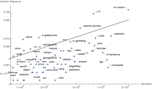
And we can see that, as expected, there is a connection between reputation and comment mentions, but a) it’s relatively weak and b) there are a number of users (most notably J.M. here) who are mentioned much more often in the comments than would be predicted directly from their reputation.
Also note that this is not total sample of all users. We are sampling only comments from a given subset of users and these comments are further dominated by a small number of users. If were were to take *all* comments I expect we would see a very different picture.
Word types
Finally, we’ll look at the types of words that are used in the comments. We’ll take a FeatureSpacePlot of the most common 100 with names longer than three letters, dropping the user names.
featWrds =
   Select[
     Complement[
       Keys@
     TakeLargest[KeySelect[comCounts, StringLength[#] > 3 &], 300],
       Take[userNames, 100]
       ],
     StringMatchQ[LetterCharacter ..]
     ];
Comment Types by Age
Comment lengths by age
Finally we’ll get to the purported point of *this* post, which was to pick apart the possible ways two people of particular ages might phrase *their* posts. Or, more concisely and with fewer word starting with p, how does age affect word choice in comments.
Let’s start by correlating our comments and ages of posters:
idImpComs =
   StringSplit[htmlImp[#], "\n\n"] & /@ idComments;

ageImpComs =
   Flatten@KeyValueMap[
      Thread[#2 ->
          idAges[Key@#]
         ] &,
      idImpComs
      ];
And again we’ll dump this on the web:
CloudExport[ageImpComs, "MX",
"stack_exchange_data/comments/mmaAgeTaggedComments.mx",
  Permissions -> "Public"
  ]

(*Out:*)

CloudObject["https://www.wolframcloud.com/objects/b3m2a1.datasets/stack_exchange_data/comments/mmaAgeTaggedComments.mx"]
We can then group these things by age to take a look at the length of the average post for a person of a given age:
ageImpGroupComs =
   GroupBy[ageImpComs, Last -> First];
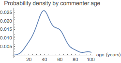
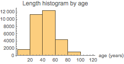
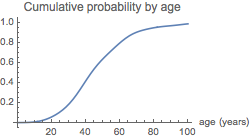
One thing to remember is that around three quarters of these posts will be been written by someone between the ages of 20 and 60, so this is the population we will primarily be probing.
ageComsWeighted =
   Map[Length, ageImpGroupComs] //
   WeightedData[Keys[#], Values[#]] &;
ageComsDist =
   ageComsWeighted //
     SmoothKernelDistribution;
ageComsCDF =
   Evaluate[
      CDF[ageComsDist, #]
      ] &;
ageComsPDF =
   Evaluate[
      PDF[ageComsDist, #]
      ] &;
ageComsCDF[60] - ageComsCDF[20]
Grid@{
   {
     Plot[ageComsPDF[x],
       {x, 0, 100},
       PlotLabel -> "Probability density by commenter age",
       AxesLabel -> {"age (years)"},
       ImageSize -> 250
       ],
     Histogram[ageComsWeighted,
       PlotLabel -> "Length histogram by age",
       AxesLabel -> {"age (years)"},
       ImageSize -> 250
       ]
     },
   {
     Plot[ageComsCDF[x],
       {x, 0, 100},
       PlotLabel -> "Cumulative probability by age",
       AxesLabel -> {"age (years)"},
       ImageSize -> 250
       ]
     }
   }

(*Out:*)

0.74258

(*Out:*)
 |  |
 | Null |
First, we’ll look at mean comment length by age. To start let’s just look at what we’re working with:
ageMeanComLens =
   Reverse@KeySort[Mean@*Map[StringLength] /@ ageImpGroupComs];
ListLinePlot[
  List @@@ Normal@ageMeanComLens,
  PlotRange -> All,
  AxesLabel -> {"user age (years)", "mean len (chars)"}
  ]

(*Out:*)
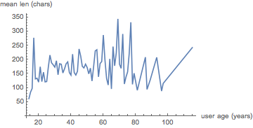
This is all pretty messy. We’ll re-bin and re-average to smooth this out, but first we’ll see what’s going on around 18:
N@KeySelect[ageMeanComLens, Between[{15, 18}]]

(*Out:*)

<|18 -> 131.912, 17 -> 277.296, 16 -> 98.1176, 15 -> 85.|>
So we see something is going on ~17. If we look at our population of 17-year-old users, we have a small number of them:
Length[
  theYouths =
    Select[Keys@idImpComs, idAges[Key@#] == 17 &]
  ]

(*Out:*)

6

{N@Mean@Map[StringLength, #], Length[#]} & /@

 Lookup[idImpComs, theYouths]

(*Out:*)

{ {108.667, 3}, {145., 10}, {110., 1}, {146.5, 2}, {280.777,
  779}, {50.5, 2} }
We see we have one very active, very chatty 17 year old who is contributing most of this. Since most people first see Mathematica in college and one would expect a 17 year old would been in his or her first semester of college, it is particularly surprising they’re so active. Just to confirm, let’s see when they made their account:
FromUnixTime@
 First@mUsers[Select[#["user_id"] == theYouths[[-2]] &],
   "creation_date"]

(*Out:*)

Which would suggest they were 12 at the time, which seems entirely implausible (and StackExchange probably doesn’t even allow that). So we’ll write them off as having their age mislabeled.
Returning to the original thread, we’ll re-bin by 5 year increments, routing through EventSeries to get the Quantity spec in.
ageComLens =
   KeySort[{Mean[#], Length[#]} &@*Map[StringLength] /@
    ageImpGroupComs];
ageComLenES =
   MovingMap[
     Mean@Flatten@
         Map[
           ConstantArray[#[[1]], #[[2]]] &,
           #
           ] &,
     EventSeries[
       KeyMap[DateObject[{2000}] + Quantity[#, "Years"] &,
     ageComLens]
       ],
     Quantity[5, "Years"]
     ];
ageComLenPlotListFull =
   Map[
     {QuantityMagnitude[Round[#[[1]] - DateObject[{2000}]]], #[[2]]} &,
     ageComLenES["DatePath"]
     ];
ListLinePlot[ageComLenPlotListFull,
  AxesLabel -> {"user age (years)", "mean len (chars)"},
  PlotRange -> All
  ]

(*Out:*)
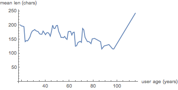
This is still quite messy (and we have a few people claiming, implausibly, to be well into their nineties or above). So we’ll ignore anything over 85 or so.
ageComLenPlotList =
   Map[
     {QuantityMagnitude[Round[#[[1]] - DateObject[{2000}]]], #[[2]]} &,
     TimeSeriesWindow[ageComLenES,
        DateObject[{2000}] + {Quantity[0, "Years"],
       Quantity[85, "Years"]}
        ]["DatePath"]
     ];
ListLinePlot[ageComLenPlotList,
 AxesLabel -> {"user age (years)", "mean len (chars)"}]

(*Out:*)
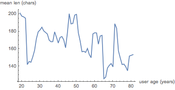
This is still quite messy, but in general, we can see from this that verbosity seems to decrease with age. Of course, we are averaging over many many more at the younger ages, so a few rather terse users in their seventies can put quite a skew on the data. This overall trend does make sense, however, with regards to recent research on how people communicate based on social status . That older people would be more comfortable being terser could be a reasonable corollary to that.
Of course, this effect is small and the underlying data is bad, but it’s a fun possible interpretation.
Comment content
Another interesting thing to look at is comment sentiment. Mathematica supports the absolute most basic sentiment analysis in Classify so we’ll first fragment our comments into sentences:
ageComSentences =
   Map[TextCases[StringRiffle[#, "\n\n"], "Sentences"] &,
   ageImpGroupComs];
Then classify all of these by sentiment. We’ll then do a simple -1, 0, 1 translation of these sentiments:
ageComSents =
   Replace[
       Classify["Sentiment", #],
       {
         "Positive" -> 1,
         "Neutral" -> 0,
         "Negative" -> -1,
         Indeterminate -> Nothing
         },
       {1}
       ] & /@ ageComSentences;
Then we’ll just look at the mean of all of these sentiments as a function of age:
ListPlot[List @@@ Normal[Mean /@ ageComSents], PlotRange -> All]

(*Out:*)
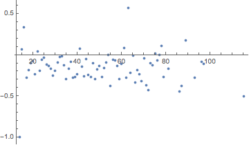
And so in general these sentiments skew a negative, but not terribly so. And that in many ways makes sense, as almost always people come to StackExchange because they have an issue they want resolved.
Next we’ll do the same binning procedure as last time to get a less noisy version of this:
ageComSentLens =
   KeySort[{Mean[#], Length[#]} & /@ ageComSents];
ageComSentES =
   MovingMap[
     Mean@Flatten@
         Map[
           ConstantArray[#[[1]], #[[2]]] &,
           #
           ] &,
     EventSeries[
       KeyMap[DateObject[{2000}] + Quantity[#, "Years"] &,
     ageComSentLens]
       ],
     Quantity[5, "Years"]
     ];
ageComSentPlotList =
   Map[
     {QuantityMagnitude[Round[#[[1]] - DateObject[{2000}]]], #[[2]]} &,
     TimeSeriesWindow[ageComSentES,
        DateObject[{2000}] + {Quantity[0, "Years"],
       Quantity[85, "Years"]}
        ]["DatePath"]
     ];
ListLinePlot[ageComSentPlotList,
  AxesLabel -> {"user age (years)", "mean sentiment"},
 PlotRange -> All]

(*Out:*)
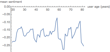
And here we find there is absolutely no connection between comment sentiment and age, belying the common stereotype of the crotchety old person. On StackExchange, instead, we are all crotchety, young and old.
Another interesting thing to look at is the spread of the sentiments. For this we’ll stack a bunch of Histogram to make a 3D plot. Just to make life more manageable we’ll group by years of five.
ageComSentsFiveGroups =
   KeySort@GroupBy[
      Normal@KeySelect[ageComSents, LessThan[85]],
      5*Quotient[#[[1]], 5, 1] & -> Last,
      Flatten
      ];
ageComSentHist =
  Histogram3D[
    KeyValueMap[
      Thread[{#, #2}] &,
      ageComSentsFiveGroups
      ],
    Automatic,
    "Probability",
    ChartStyle -> {Opacity[1], Automatic}
    ]

(*Out:*)
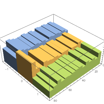
And here we can see there might actually be age-dependent trends each different sentiment that were cancelling in the mean.
For those interested, I’ve dumped this plot here:
CloudDeploy[
  ageComSentHist,
  "stack_exchange_data/comments/mmaCommentsAgeSentiments.nb",
  Permissions -> "Public"
  ]

(*Out:*)

CloudObject["https://www.wolframcloud.com/objects/b3m2a1.datasets/stack_exchange_data/comments/mmaCommentsAgeSentiments.nb"]
Once the cloud supports all Graphics3D primitives that will be viewable in 3D. For now you can always download the notebook with CloudImport
Age vs Individual Sentiments
The most striking progression in that seems to be the decrease in positive sentiment in posts with age, so we’ll start by looking at that:
ageComSentsPosLens =
   KeySort[{Length[Cases[#, 1]], Length[#]} & /@ ageComSents];
ageComSentPosES =
   MovingMap[
     Total[#[[All, 1]]]/Total[#[[All, 2]]] &,
     EventSeries[
       KeyMap[DateObject[{2000}] + Quantity[#, "Years"] &,
     ageComSentsPosLens]
       ],
     Quantity[5, "Years"]
     ];
ageComSentPosPlotList =
   Map[
     {QuantityMagnitude[Round[#[[1]] - DateObject[{2000}]]], #[[2]]} &,
     TimeSeriesWindow[ageComSentPosES,
        DateObject[{2000}] + {Quantity[0, "Years"],
       Quantity[85, "Years"]}
        ]["DatePath"]
     ];
ListLinePlot[ageComSentPosPlotList,
  AxesLabel -> {"user age (years)", "percent positive"},
 PlotRange -> All]

(*Out:*)
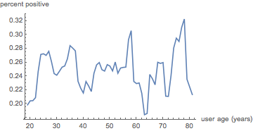
With this better sampling procedure much of what we saw before disappears. We can still check, though, what happens when plot all three sentiments simultaneously:
ageComSentsNeutLens =
   KeySort[{Length[Cases[#, 0]], Length[#]} & /@ ageComSents];
ageComSentNeutES =
   MovingMap[
     Total[#[[All, 1]]]/Total[#[[All, 2]]] &,
     EventSeries[
       KeyMap[DateObject[{2000}] + Quantity[#, "Years"] &,
     ageComSentsNeutLens]
       ],
     Quantity[5, "Years"]
     ];
ageComSentNeutPlotList =
   Map[
     {QuantityMagnitude[Round[#[[1]] - DateObject[{2000}]]], #[[2]]} &,
     TimeSeriesWindow[ageComSentNeutES,
        DateObject[{2000}] + {Quantity[0, "Years"],
       Quantity[85, "Years"]}
        ]["DatePath"]
     ];
ageComSentsNegLens =
   KeySort[{Length[Cases[#, -1]], Length[#]} & /@ ageComSents];
ageComSentNegES =
   MovingMap[
     Total[#[[All, 1]]]/Total[#[[All, 2]]] &,
     EventSeries[
       KeyMap[DateObject[{2000}] + Quantity[#, "Years"] &,
     ageComSentsNegLens]
       ],
     Quantity[5, "Years"]
     ];
ageComSentNegPlotList =
   Map[
     {QuantityMagnitude[Round[#[[1]] - DateObject[{2000}]]], #[[
      2]]} &,
     TimeSeriesWindow[ageComSentNegES,
        DateObject[{2000}] + {Quantity[0, "Years"],
       Quantity[85, "Years"]}
        ]["DatePath"]
     ];
ListLinePlot[
  {
    ageComSentPosPlotList,
    ageComSentNeutPlotList,
    ageComSentNegPlotList
    },
  AxesLabel -> {"user age (years)", "percent sentiment"},
  PlotRange -> All,
  PlotLegends -> {"positive", "neutral", "negative"}
  ]

(*Out:*)
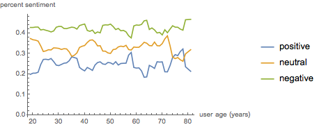
And here we see something interesting. Negative sentiment was pretty constant across ages, but the except in a few instances (I’m looking at you, 55 and 62 year olds), positive and neutral sentiments were coupled.
What this means I have no idea, but it is an interesting result none-the-less.
Verbosity vs Sentiment
One might be interested in whether the two trends we’ve looked at, verbosity and sentiment, are connected. We can plot this by pulling from these plot lists and doing a direct correlation:
ListPlot[
  Thread[
    {
      ageComLenPlotList[[All, 2]],
      ageComSentPlotList[[All, 2]]
      }
    ],
  AxesLabel ->
    {
      "mean len (char)",
      "mean sentiment"
     }
  ]

(*Out:*)
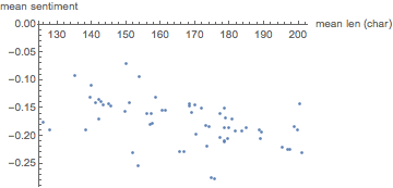
And that’s a decently convincing connection between increasing mean comment length and sentiment. We can quantify the fit like so:
sentFit =
  LinearModelFit[
    Thread[
      {
        ageComLenPlotList[[All, 2]],
        ageComSentPlotList[[All, 2]]
        }
      ],
    chars,
    chars
    ]

(*Out:*)

So we get a weak-negative correlation between comment length and sentiment. Then we can pull the goodness-of-fit:
sentFit["RSquared"]

(*Out:*)

0.218534
And yes, this is a pretty terrible fit, but much better than one might expect for such a messy set of data.
Conclusions
With all of that, I think this has gone on long enough, but we can restate some basic conclusions we found.
-
We can model the expected length of a comment by considering three terms: 1) a standard
GammaDistributionthat models a basic discrete, always positive process 2) a very broadNormalDistributionthat captures the breadth of comment distributions 3) a very small, sharpNormalDistributionthat recovers the fact that there is a limit to comment lengths and many people will push right up to it. -
The standard language used on the stack exchange skews towards bug-fixes and workarounds, as compared to standard English. This might tell us something about how buggy and how many dark corners a huge chunk of software like Mathematica can have.
-
Reputation and comment mentions are directly correlated, but some people are particularly highly mentioned for their rep. This could easily be an artifact of the dataset, or it could describe relative proclivities for conversing in the comments.
-
User age and mean comment length are negatively correlated, while user age and mean comment sentiment have no connection whatsoever.
-
Negative sentiment as expressed in comments is largely constant across ages, but positive and neutral sentiment are reasonably closed coupled, causing the dynamics we saw in the mean sentiment analysis
-
Mean comment length and mean comment sentiment are negatively correlated with each other. What causes this is anyone’s guess, but it’s, at minimum, and interesting correlation