Quantum Chemistry in Mathematica, A DVR Framework
This will (time-permitting) be the first of a series of posts on doing quantum chemistry in Mathematica. This post will focus on one of the simplest non-standard techniques for solving the Schrödinger equation, called discrete variable representation (DVR).
A Discrete Variable Representation Framework
Discrete variable representation (DVR) as a technique for computing wavefunctions dates back to some time in the ‘60s, but didn’t really get much attention until John Light and coworkers started to use it in the ‘80s. For those interested, Light and Carrington published a review paper in 2003 called Discrete Variable Representations and their Utilization that provides a more in-depth look at DVR and its history.
DVR is a grid-based method, which is based off of two approximations:
-
The basis-functions are localized at the grid points
-
Gaussian quadrature can be used to exactly compute the requisite integrals for a matrix representation of the Hamiltonian
These approximations come from the realization that families of classical orthogonal polynomials have associated quadrature points, which can be used as a grid for an exact representation the Hamiltonian.
Why DVR?
DVR has two desirable characteristics in terms of simplifying chemical problems:
-
Functions in pure coordinates have diagonal matrix representations (i.e. there is no coupling between grid points)
-
Matrix representations in a DVR are very sparse
The first of these means that we can simply use Psi4 or Gaussian to generate evaluate the potential at the grid points when building up a representation of the potential. The second means that we can use efficient iterative methods for diagonalizing the Hamiltonian. An unfortunate complication is that the kinetic energy may not have a simple statement in the DVR basis, but given the age of the technique, many complicated operators have already been represented in standard DVR bases.
DVR is also good for the programmer, as its simple and modular. The most computation intensive aspects of working with DVR are generating a representation for the kinetic energy and diagonalizing the Hamiltonian. With a semi-modern laptop (2012 MacBook Pro), even for complex systems, both of these can be done locally in under 30 minutes.
The modularity makes frameworking convenient, as there are always 4 steps that need to be done:
-
Generate the coordinate grid
-
Use the grid to generate the kinetic and potential matrices
-
Add these and diagonalize to get the wavefunctions
-
View the wavefunctions
Of these, often only the grid and kinetic energy need to be changed (and sometimes not even the former) when implementing a new DVR scheme.
Even better, multi-dimensional DVRs are often implemented as direct products of one-dimensional DVRs, which allows such a framework to reap double the benefits
A DVR Object System
Our DVR framework will be based on a concept of “classes” of DVRs and “instances” of these DVR classes. As an example, in a 1984 paper , Daniel Colbert and William Miller introduced a DVR scheme that works on the range [-∞, ∞]. A general implementation of that scheme would be a DVR class on a 1D Cartesian grid. An instance of that DVR class would be a specific DVR using 151 grid points on the range [-2, 2].
At this point, I’ve written DVR classes for a number of general cases. First, we’ll load the DVR submodule of my ChemTools package:
Needs["ChemTools`DVR`"]
If you need to install ChemTools to you can get it like so:
PacletInstall["ChemTools",
  "Site" ->
  "http://www.wolframcloud.com/objects/b3m2a1.paclets/PacletServer"
  ]
Then we can list the classes available:
ChemDVRClasses[]

(*Out:*)

{"Cartesian1DDVR", "LegendreDVR", "MeyerDVR", "PlanePointDVR", \
"ProlateTopDVR", "RadialDVR", "SlowLoadingDVR", "SphericalDVR"}
The DVR we’ll be using here is what I called the "Cartesian1DDVR" . We’ll first load the class:
c1ddvrclass = ChemDVRClass["Cartesian1DDVR"]

(*Out:*)
Then we can use the class to build an object:
c1ddvr = c1ddvrclass[]

(*Out:*)

This is now a proper object we can play with. It comes pre-populated with a harmonic oscillator potential, and we can see how it looks on that (note we’re using Manipulate -> False for static display purposes):
c1ddvr[Manipulate -> False]

(*Out:*)
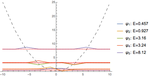
This approximation is super rough. Let’s polish it up a bit by using more points:
c1ddvr[
  "Points" -> {151},
  Manipulate -> False
  ]

(*Out:*)
This is a good approximation. And it’s fast. Let’s generate interpolating versions of the first few of these:
c1ddvr[
  "Points" -> {151},
  Return -> "InterpolatingWavefunctions",
  "WavefunctionSelection" -> ;; 5,
  Manipulate -> False
  ]

(*Out:*)
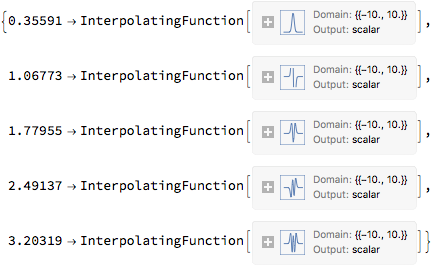
This gives us wavefunction energies and interpolating functions.
Double-Well Potential
That’s fun, but the harmonic oscillator is a little boring. Let’s play with a more interesting potential (but not too interesting, mind you). We’ll do a half-square, double-well potential.
L = 10;
barR = barL = 10000;
v0 = L(*^-1.5*);
zp = 0;
pot =
  Compile[{ {x, _Real} },
    With[{L = L, v0 = v0, zp = zp, barR = barR, barL = barL},
      Piecewise[{
         {barL,
           x < L (-3/2)},
         {zp,
           L (-3/2) <= x <= L (-1/2)},
         {v0,
           L (-1/2) < x < 0},
         {v0*Power[1 - Exp[(x - L)*Power[x, -.5]], 2],
           0 <= x}
         }]
      ],
    RuntimeOptions -> {
       "EvaluateSymbolically" -> False
       }
    ]

(*Out:*)
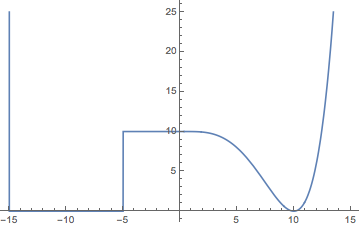
We’ll quickly confirm we have a nice double-well:
Plot[pot[x], {x, -(3/2 + 1/100) L, (3/2 + 1/100)*L }]

(*Out:*)
And then we’ll feed this into a new DVR object on a new range.
c1ddvr2 = c1ddvrclass[{151}, {2 L*{-1, 1}}];

c1ddvr2[
  Function -> pot,
  Manipulate -> False,
  "WavefunctionSelection" -> 3,
  PlotRange -> {-.1, .5}
  ]

(*Out:*)
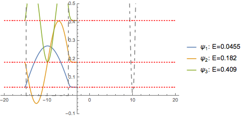
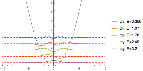
We can see that it appears as if we have standard particle-in-a-box wavefunctions on the left (1 and 3) and Morse-oscillator functions on the right (2). We can then extract the "InterpolatingWavefunctions" :
wfns = c1ddvr2[Function -> pot,
   Return -> "InterpolatingWavefunctions"];
Then we can Animate these:
ListAnimate[
  MapIndexed[
    Show[
       Plot[Evaluate[#[[1]] + #[[2]][x]], {x, -2 L, 2 L},
         PlotRange -> {-.1, 10 + #[[1]]},
         PlotStyle -> ColorData[97][#2[[1]]]
         ],
       Plot[pot[x], {x, -2 L, 2 L},
     PlotStyle -> Directive[Dashed, Gray]]
       ] &,
    Take[wfns, 25]
    ]
  ]

(*Out:*)
Other DVR Schemes
Many different types of DVRs are possible. I have constructed DVRs in up to 3 dimensions, although theoretically arbitrary dimensional DVRs are possible. Similarly I’ve constructed DVRs that work in angular coordinates, or which are appropriate for radial wavefunctions (which allowed me to build a DVR on a spherical grid). For now, though, we’ll leave it at this and come back to those some other day.