Psi4 4 Mathematica

We’ll return to doing fake chemistry , but this time we’ll work with something that very real chemists have built, namely the open-source quantum chemistry package Psi4 the package itself is voluminous, doing many things I don’t understand and never really will, but it does do some things that every chemist knows and many use or at the minimum enjoy looking at–molecular orbitals and electric potentials.

Here’s a taste of the sort of thing we’re talking about:

AtomsetOrbitalsPlot[trifluoromethlyoxirane,
  "Orbitals" -> {5},
  "Mode" -> "Cached"
  ]

(*Out:*)

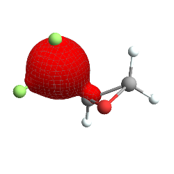
This is the 5th molecular orbital of trifluoromethyl-oxirane , more or less, plotted as a ContourPlot3D (with stylistic choices taken from Jason Biggs ) in Mathematica. Note that things are slightly askew – the lobes and the reference molecule don’t perfectly align, but this is a pretty reasonable orbital, all told. So first let’s break down how this was made, starting with the easiest bits (if you just want the Psi4 integration bits go here ):

‌

Making Trifluoromethyl oxirane

Generally when I play around with this stuff I do it by using stuff I can directly import–-and I did test this code using importable cases—but, for interest sake, I thought I’d try working with a system I knew about but wasn’t importable.

On the other hand it’s mostly importable:

ChemImport[methyloxirane] // ChemView

(*Out:*)

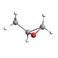
And so we only have to do, say, two things:

• Replace the methyl hydrogens with fluorines

• Renormalize those bonds

And we could do this in a lazy sort of way, say:

• Find the hydrogens

• Remove the hydrogens

• Create 3 fluorines

• Move the fluorines in, rebond, etc.

• Calculate fluorine bond vectors, move them along the vector back into place

But this is a lot of work for just trifluoromethly-oxirane and this sort of operation is just generally pretty useful, so we’ll functionalize it in three chunks:

• Atom selection by type (e.g. methyl hydrogen)

• Atom substitution

• Atomset bond normalization

Atom Selection

This is a more interesting problem in general, really, than just the case of methyl groups, as it can be generalized pretty easily to any group with a core atom. We can basically think of specifying such a group as the following:

<|
  "Core" -> type,
  "Bonds" -> {
     <|"Element" -> el1, "Type" -> type1|>,
     <|"Element" -> el2, "Type" -> type2|>,
     ...,
     <|"Element" -> eln, "Type" -> typen|>
     }
  |>

Or more compactly:

type ->
  {
    el1 -> type1,
    el2 -> type2,
    ...,
    eln -> typen
    }

And then a methyl group is just:

"C" ->
  {
    "H" -> 1,
    "H" -> 1,
    "H" -> 1,
    _
    }

Since we can (and in fact should) write this to leverage Mathematica’s pattern specifications / matching. And one last thing we’ll find very useful is the ability to add a selection specification to what we’ll take. We’ll let this be a general pattern that will match against the atom type. So for our methyl hydrogens:

"C" ->
  {
     "H" -> 1,
     "H" -> 1,
     "H" -> 1,
     _
     } -> "H"

Simple enough to specify. Now the implementation isn’t too bad, the primary difficulty is to do it in a chunked fashion. Essentially pull in all the data at the beginning rather than at each loop step. The full implementation isn’t worth putting here, but you can find it under AtomsetAtomMemberQ in Objects.m essentially after all that we can select atoms that are members of groups in atomsets and there are a few cooked in. What’s relevant right now is how this works for methyl hydrogens:

AtomsetGetAtoms[methyloxirane, "Methyl" -> "H"] // ChemView

(*Out:*)

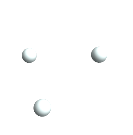
Basically the "Methyl" says, “find atoms in methly groups” and the "H" says only take the hydrogens from that group. And lo and behold it works. On to part 2.

Atom Substitution

This is honestly the easiest part of the whole deal. It’s almost as straightforward as can be, easy to vectorize, etc. The basic part is to set the positions of the new atoms to those of the old atoms:

 AtomsetRemoveAtom[obj, old];
 AtomsetAddAtom[obj, new];
 pos = ChemGet[old, "Position"];
 ChemThreadSet[new, "Position", pos];

Then do the bonds:

BondBreak /@ DeleteDuplicates@Flatten@bonds;
types = ChemGet[bonds, "Type"];
atoms =
   Replace[
     ChemGet[bonds, "Atoms"],
     ({Alternatives @@ old, a_} | {a_, Alternatives @@ old}) :> a,
     {2}
     ];

And just MapThread a mapped AtomCreateBond over that.

Bond Normalization

This is the fun part. First of we need a concept of what the “standard” distance is for all these bond types. I’ve accumulated a number of those, by statistically going through PubChem and averaging over bond types. This is integrated into ChemDataLookup .

ChemDataLookup[ChemDataQuery["C", "F"], "BondDistances"]

(*Out:*)

1.34782

Where these distances should be Quantity expressions with units "Angstroms" . But I’m lazy and that adds a mild inefficiency. So we’ll let that be our standard. Note that if there wasn’t a distance in the sample I used we’re screwed:

ChemDataLookup[ChemDataQuery["Ne", "F"], "BondDistances"]

(*Out:*)

-1.

Also some of these are slightly odd:

ChemDataLookup[ChemDataQuery["S", "F"], "BondDistances"]

(*Out:*)

1.19224

But for common cases things are okay. And this data will be updated periodically when time permits.

ChemDataLookup[
  {
    ChemDataQuery["C", "H"],
    ChemDataQuery["C", "O"],
    ChemDataQuery["C", "N"],
    ChemDataQuery["C", "C"],
    ChemDataQuery["C", "C", 2],
    ChemDataQuery["C", "C", 3]
    },
  "BondDistances"
  ]

(*Out:*)

{1.02348, 1.29987, 1.42094, 1.42432, 1.35593, 1.2004}

So that’s our normalization. Now we have to figure out what needs to be normalized. We’ll do this by comparing against a tolerance set by the AccuracyGoal option, where anything whose bond length deviates from the standard by more than that gets normalized.

And now here’s the interesting part. If we, say, normalize any of the C-C bonds in methyl-oxirane that will screw up all sorts of other bonds. In effect, we need to move one “side” of the bond by the amount of deviation. Where each “side” is really the collection of connected atoms that don’t use the bond. A good example of what I mean is in the documentation for AtomsetConnectedComponents .

We’ll do this by building an AtomGraph of all the atoms in the atomset, taking the edges, and then for each bond we normalize dropping the edge corresponding to it. Then use a simple ConnectedComponents on that to find our “sides”. Of course, one corner case arises here. Consider this:

Graph[
  {
    1 <-> 2,
    2 <-> 3,
    3 <-> 4
    }
  ]

(*Out:*)

Now drop the 1 <-> 2 bond:

Graph[
   {
     2 <-> 3,
     3 <-> 4
     }
   ] // ConnectedComponents

(*Out:*)

{ {2, 3, 4} }

We’ve lost the knowledge about 1. So we need an explicit check for that at each loop-step. But otherwise we just need to determine which side is which by figuring out which chunk contains the first atom in the bond.

Then just move each side equally and in opposite directions so that the tolerance is dealt with.

Note, of course, that there are some structures, notably ringed structures, for which this method will not suffice. But for most small-molecules, like trifluoromethly-oxirane, this will.

Now for a demonstration:

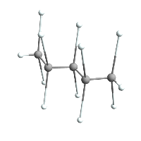
ChemImport[pentane];
AtomsetTransform[pentane, ScalingTransform[{1, 1, 3}]];
pentane // ChemView

(*Out:*)

AtomsetNormalizeBonds[pentane]
pentane // ChemView

(*Out:*)

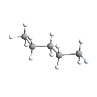
And now checking the bond deviations:

BondDeviation@Values@AtomsetBonds[pentane]

(*Out:*)

{0., 0., 2.22045*10^-16, 
 2.22045*10^-16, 0.0963753, -6.66134*10^-16, -4.44089*10^-16, \
0.096458, -6.66134*10^-16, 2.22045*10^-16, 
 1.77636*10^-15, -1.55431*10^-15, 0.0718594, 
 1.77636*10^-15, 0.0717659, 4.44089*10^-16}

They’re mostly all 0, except for 4 of them, and we can see which those are:

Pick[
     #,
     # > .01 & /@ Abs[BondDeviation[#]]
     ] &@Values@AtomsetBonds[pentane] // ChemView

(*Out:*)

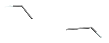
And those are bonds that are in the plane of the chain, and so were likely unscaled by the ScalingTransform . That the other two bonds were caught up could be an effect of the odd C-C bond distance I have in my core data, too.

Making a trifluoromethly-oxirane

And finally with that in place, build and substitute:

trifluoromethlyoxirane = ChemImport["methyloxirane"];
subs = Table[CreateAtom["F"], 3];
AtomsetSubstituteAtom[
   trifluoromethlyoxirane,
   Thread[
     AtomsetGetAtoms[trifluoromethlyoxirane, "Methyl" -> "H"] ->
      subs
     ]
   ];
tfgraphic = trifluoromethlyoxirane // ChemView

(*Out:*)

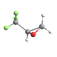
And renormalize:

subbonds =
   DeleteDuplicates@
     Flatten@
       ChemGet[
         AtomsetGetAtoms[trifluoromethlyoxirane,
           "C" -> { "F" -> _, "F" -> _, "F" -> _, _ } -> "F"
           ], 
         "Bonds"
         ];
AtomsetNormalizeBonds[
   trifluoromethlyoxirane,
   subbonds
   ];
Show[trifluoromethlyoxirane // ChemView, tfgraphic]

(*Out:*)

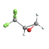
And of course we can easily do the same for, say, tribromomethyl-oxirane, which doesn’t seem to have a Chem Spider page:

tbmo = ChemImport["methyloxirane"];
subel = "Br";
subs = Table[CreateAtom[subel], 3];
AtomsetSubstituteAtom[
   tbmo,
   Thread[
     AtomsetGetAtoms[tbmo, "Methyl" -> "H"] ->
      subs
     ]
   ];
subbonds =
   DeleteDuplicates@
     Flatten@
       ChemGet[
         AtomsetGetAtoms[subel,
           "C" -> { subel -> _, subel -> _, subel -> _, _ } -> subel
           ], 
         "Bonds"
         ];
AtomsetNormalizeBonds[
   tbmo,
   subbonds
   ];
tbmo // ChemView

(*Out:*)

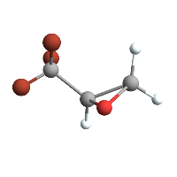
Or on anything with a methyl group.

‌

Psi4’s The 1 4 me

One of the many nice features of Psi4 is that it’s implemented in C++ rather than Fortran, so not only is the code easily readable to anyone with a decent grounding in modern programming languages ( Java, python, JavaScript, any other C-flavored language). Moreover, that makes it possible to use with Library Link if one so desired. This I did not do. Instead I decided to build a symbolic python system to use with Psi4’s Psithon interpreter. The vagaries of this system are convoluted and not worth going into here. Here’s just a quick example of what it provides:

Needs["ChemTools`SymbolicPython`"];
sympy =
  ToSymbolicPython[
    Map[f, Range[100]]
    ]

(*Out:*)

PyList[PyMap["f", PyRange[100]]]

And we can build this out like so:

sympy // ToPython

(*Out:*)

"list(map(f, range(100)))"

The symbolic layer is useful as a transform and whatnot, and is also a cleaner syntax to write templates in than strings. And it can be used for OpenBabel too.

So with that in hand we can actually get around to writing stuff to play with Psi4

CubeProp

Psi4 has a module that implements calculations that dump to a Gaussian cube file called cubeprop it’s pretty straightforward and most cubeprop calls have a similar set-up. So we’ll mirror that in our template code and build out a general purpose function called Psi4CubeProperty to implement this transformation.

psi4In = Psi4CubeProperty[<|"Molecules" -> { {"O"} }|>]

(*Out:*)

It generates an input file to push through psithon:

psi4In["input.dat"]

(*Out:*)

"#Sat 29 Jul 2017 02:13:19\n#Cube prop call\nmolecule monomer {\n\tO \
0. 0. 0.\n\tnoreorient\n\tnocom\n\t}\nset {\n\tbasis cc-pvdz\n\t\
scf_type df\n\tcubeprop_tasks orbitals\n\tcubeprop_orbitals [ 1 ]\n\t\
}\n[ E, wfn ] = energy('scf', return_wfn=True)\ncubeprop(wfn)"

So that’s cool. And then we implement layers on that function for specific useful tasks. For example here’s the code that builds out an orbitals call.

Options[Psi4CubeOrbitals] = Options@Psi4CubeProperty;
Psi4CubeOrbitals[a_Association] :=
   Psi4CubeProperty@
     Merge[{
        Append[a,
          
      "Configuration" ->
            
       Merge[{Lookup[a, "Configuration", <||>],
               <|
                 "CubePropTasks" -> {"orbitals"},
                 
          "CubePropOrbitals" -> {1, -1, 2, -2, 3, -3, 4, -4, 5, -5}
                 |>
               },
              First]
          ],
        "Output" -> "Psi_*.cube"
        },
       First];
Psi4CubeOrbitals[atomList_List, orbitals : {__Integer} : {1}, 
   p : (_Rule | _RuleDelayed) ...] :=
   Psi4CubeOrbitals@
     <|
       "Molecules" -> atomList,
       "CubePropOrbitals" -> orbitals,
       p
       |>;
Psi4CubeOrbitals[atomList_List, orbitals_Integer, 
  p : (_Rule | _RuleDelayed) ...] :=
  
 Psi4CubeOrbitals[atomList, Join[#, -#] &@Range[orbitals]]

The options handling gets a bit convoluted, but otherwise it’s really very standard. And then we build a layer on the atomset side to call Psi4 to get these orbitals:

AtomsetOrbitalsPlot[
  trifluoromethlyoxirane,
  "Orbitals" -> {1},
  "Mode" -> 
  "Cached" (* tells the system to save the computed orbital functions \
*)
  ]

(*Out:*)

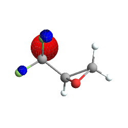
And this can, of course, be configured for arbitrary set ups.

Cube Files

One complication does arise, though, in that we need a way to handle Gaussian cube files. So I wrote a collection of CubeFile* functions that handle most of this dirty work. For each cube file what actually gets pushed through to the end is an InterpolatingFunction over the cube, so we could actually do funky things like this:

oneminustwo =
   With[{orbs =
       Values@
         AtomsetOrbitals[
           trifluoromethlyoxirane,
           "Orbitals" -> 2,
           "Mode" -> "Cached"
           ]
      },
     Compile[{ {p, _Real, 1} },
       orbs[[1]][p] -
         orbs[[2]][p]
       ]
     ];
AtomsetOrbitalsPlot[
  trifluoromethlyoxirane,
  {oneminustwo}
  ]

(*Out:*)

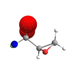
Which is the subtraction of two orbitals. This is obviously just a basic example, but there is power in being able to work with these orbitals as the functions that they are.

Alternatively we can do this plot as a ListDensityPlot3D :

AtomsetOrbitalsPlot[
   trifluoromethlyoxirane,
   {oneminustwo},
   "PlotFunction" -> "Density"
   ] // Rasterize(*to speed up rendering since we don't need to \
manipulate it*)

(*Out:*)

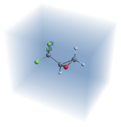
And it’s harder to see exactly what’s happening. But we can see the two super localized blobs near those two fluorines.

Electric Potentials

Psi4 exposes a lot more than just the cubeprop module, but most of that will have to wait for another post (and likely some more development on my side). One final fun thing to look at, though, is comparing electric potentials across similar.

We can start with the first-approximation Gasteiger version:

AtomsetElectricPotentialMap[#, "Mode" -> "Gasteiger"] & /@ {
    methyloxirane,
    trifluoromethlyoxirane,
    tbmo
    } // GraphicsRow

(*Out:*)

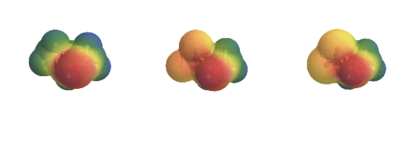
It’s a bit small, but we can see pretty clearly that it’s doing a decent job. All of that seems reasonable. But let’s just see what the real version looks like:

AtomsetElectricPotentialMap[#, "Mode" -> "Psi4"] & /@ {
    methyloxirane,
    trifluoromethlyoxirane,
    tbmo
    } // GraphicsRow

(*Out:*)

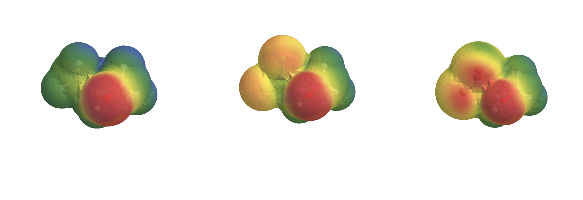
It takes a lot longer, but the quality of the result is better. This is an electric potential we can actually start to work with. And, in fact, since we have it as an InterpolatingFunction we easily could manipulate these potentials and compare them on a point-by-point basis.

But for now we’ll leave things as they are and come back to Psi4 another day.