PJLink - Hooking up Mathematica and Python

Mathematica is an incredibly powerful platform with a fun and intellectually pleasing language, but is incredibly expensive, closed source, and Stephen Wolfram rubs many people the wrong way. Python is a convenient, pretty powerful language with a lot of support from the developer community. For as long as the two have existed people have been trying to tie them together, but very little has been done to do so at the native level with efficient, convenient exchange between the two. That’s why over the past few weeks I took the time to build a clean, convenient link between the two. This post will go into how the link was built and some of its features, but first I think a little demo is appropriate.

‌

A Quick Demo

Installing PJLink

The link is based off of the J/Link interface built into Mathematica for hooking up Java and Mathematica. To wit, I called it PJ/Link . It lives on my paclet server as well as GitHub, so we can easily install it from there:

PacletInstall["PJLink", "Site"->"http://www.wolframcloud.com/objects/b3m2a1.paclets/PacletServer"]

(*Out:*)

Loading PJLink in Jupyter

For this demo we’ll need the path to this thing as well (note that the version might change in the future):

%["Location"]

(*Out:*)

"~/Library/Mathematica/Paclets/Repository/PJLink-1.0.0"

Now we’ll leave Mathematica and open up a Jupyter notebook:

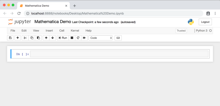
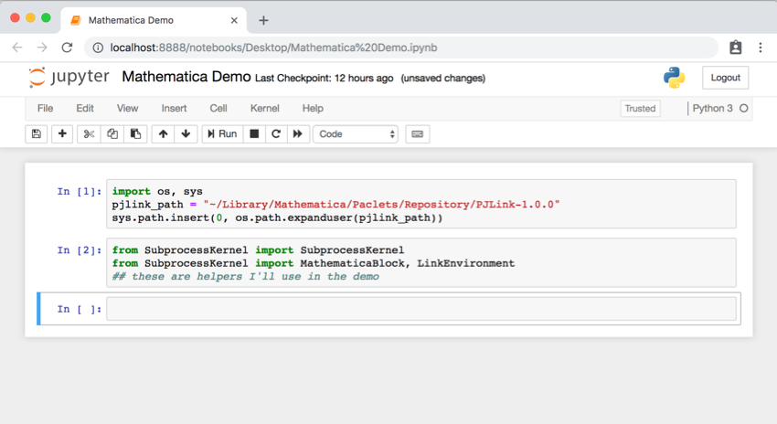
Next we’ll get that path available so we can actually make use of the package. Then we’ll load things from the subsidiary SubprocessKernel package which is included in the paclet and makes use of PJLink:

import os, sys
pjlink_path = "~/Library/Mathematica/Paclets/Repository/PJLink-1.0.0" #this is whatever path was extracted before
sys.path.insert(0, os.path.expanduser (pjlink_path))

from SubprocessKernel import SubprocessKernel
from SubprocessKernel import MathematicaBlock, LinkEnvironment
## these are helpers I' ll use in the demo

Bidirectional Communication

Once we have this we can start a subprocess kernel which will open a Mathematica front-end to interact with. We’ll also start and evaluator Mathematica can use to call back into python.

You may see a long string of output from your C compiler as the setup.py file builds out the native library that PJLink uses. Don’t worry, this should only happen once. If it fails, raise an issue on GitHub so I can deal with it.

Once Mathematica has loaded, we’ll use the MathematicaBlock context manager so we can write something that looks a lot like Mathematica code and use the MEval function we’ll define to run the code. That code for all this looks like:

ker = SubprocessKernel()
def MEval (expr, wait = True, kernel = ker) :
     "" "MEval evaluates a Mathematica expression in the Mathematica kernel
      
      " ""
    kernel.drain() # just to make sure things are clen
    return kernel.evaluate (expr, wait = wait)
ker.start()
ker.start_evaluator()

After that we can simply call into Mathematica:

with MathematicaBlock():
      res = MEval (Set (M.hi, "Hello from python!"))
res

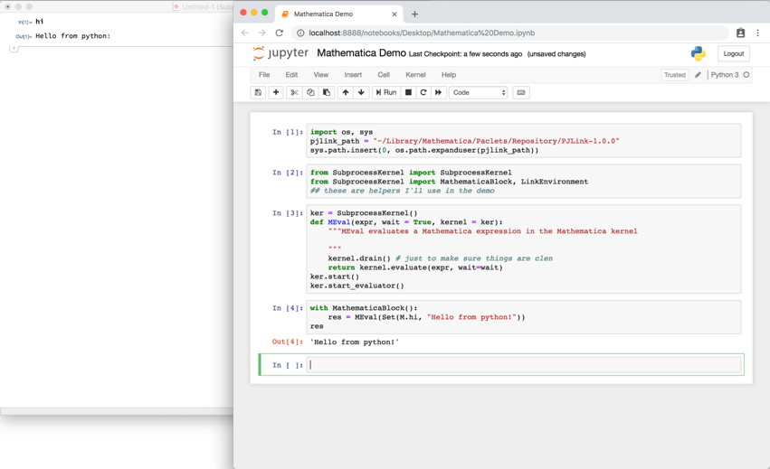
We can see string "Hello from python!" was set to the symbol hi on the Mathematica side and was returned back by MEval . Symbols that aren’t in the "System`" context need to be prefaced by an M. as that’s a special class that can resolve symbol names like that.

We can also get efficient data transfer of arrays from either side. Here we’ll take some Mathematica data and get it back out on the python side. The first thing we need to do is go to the Mathematica notebook that opened and load the "PJLink`" context. Then we’ll install the python runtime that the SubprocessKernel object configured. This looks like:

<<PJLink`
InstallPython[ LinkObject->SubprocessKernel`$PyEvaluateLink, ProcessObject->None];

Once it’s installed, we’ll use it directly via PyEvaluate :

With[{arr= RandomReal[{-1, 1}, {50, 50, 50}]},
  PyEvaluate[dat=arr]
  ]

Calls into python are done in an environment held only by the link, so to access that we need to wrap the evaluator we started ( ker.evaluator ) in a LinkEnvironment context manager:

with LinkEnvironment(ker.evaluator):
      res = dat.shape
res

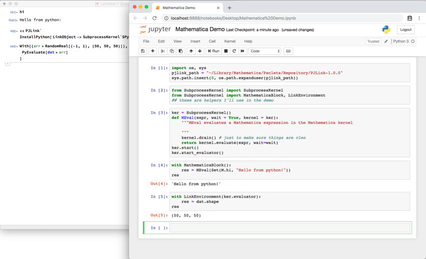
Arrays are held as NumPy arrays by default on the python side, although this may be disabled. If disabled, they’re held as a data type called BufferedNDArray which holds the data as a single C-contiguous array and allows slicing and viewing into it (although no efficient math or manipulation of any sort).

Finally, to close out the demo, we’ll plot something on the Mathematica side and watch it come back on the python side. The code for this should be pretty self-explanatory by this point, but there is one cute feature to note:

with MathematicaBlock():
      res = MEval(
           Rasterize(
                 Plot(Sin (M.x), List (M.x, 0, Times (2, Pi)),
                       ImageSize = [250, 250],
                       PlotLabel = "sin(x) as plotted in Mathematica"
                       )
                 )
           )
res

Unfortunately it really does matter that we pass a List expression instead of a python list for the second argument to Plot as otherwise the system hangs for reasons that aren’t totally clear. On the other hand, we can see how nice options passing is in the interface. We make use of the python **kwargs setup and that ImageSize= ... and PlotLabel= ... both get automatically converted into rules (albeit with a String key instead of a Symbol ). The Rasterize is, sadly, similarly necessary as there is currently no logic in the package to automatically convert Graphics expression into their rasterized forms.

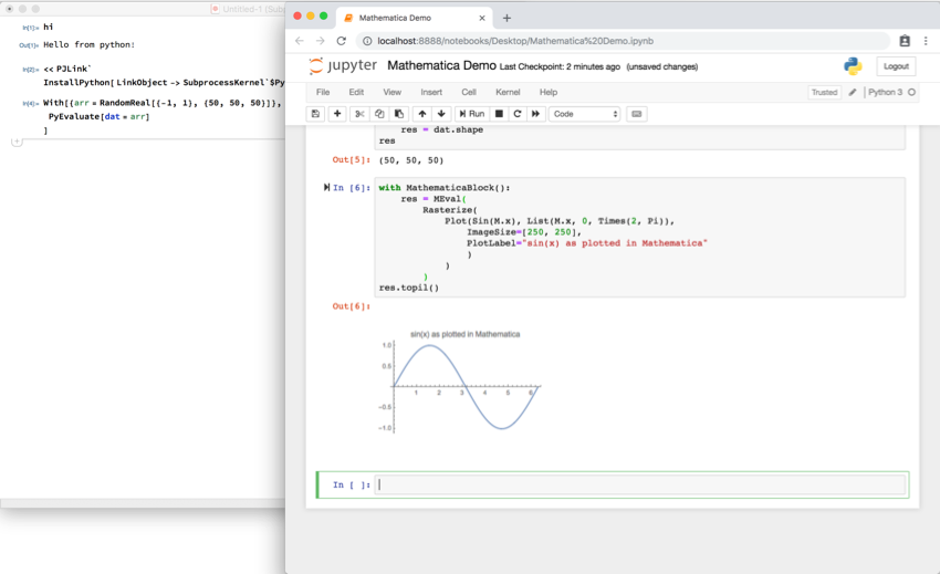
I think we’ll close out the demo here, though, and move onto a description of how this works.

‌

PJLink Native Library

The heart of PJLink is the C library that connects a python runtime to MathLink. The source for this can be found here . This library, once compiled by the setup.py file packaged with it, implements the basic MathLink calls in a way that python can use them and attempts to do so with efficient memory usage and data transfer.

Data Sharing in the Native Library

The heart of the native library is the set of PutArray and GetArray functions it implements. Beyond anything else, it is the fast transfer of large arrays of data that makes a C-level connection so appealing. The way we handle this on the python side is via the python buffer protocol . We enforce the condition that all data sent and received on the python side must be handled by an object that can work with a C-contiguous buffer of data. By default this is done with NumPy if it is installed, but if not there is a custom object called BufferedNDArray in the HelperClasses package that deals with this.

Threading in the Native Library

Python has something called the Global Interpreter Lock (GIL) which is a method for synchronizing python state. Unfortunately for us, the presence of the GIL means that standard C calls of the kind we’ll be using will cause all threads to lock. To get around this, every call into the MathLink library in the native library is wrapped in the MLTHREADED macro which handles the releasing and reacquiring of the lock. This allows our threads to work once more. Any extensions to the library should keep this in mind.

‌

Class Structures

PJLink provides a glut of classes that handle the details communication, so we will quickly detail what the important ones do. More information is always available upon request.

The *Link classes

PJLink is based off of JLink and so it makes use of the same kind of class structure that JLink does. This means that it has a MathLink class that provides a template for the kind of link we’ll work with and a KernelLink class that works specifically with Mathematica kernels. In general, we will only really work with a subclass of a KernelLink called a WrappedKernelLink that implements the KernelLink interface by calling into a NativeLink which is the only class which actually touches the native library at all.

If one is controlling a Mathematica kernel from python, it will be handled by a WrappedKernelLink .

Reader class

The Reader class handles the other half of the communication. It waits for calls from Mathematica and processes them via the KernelLink._handlePacket function. Most commonly these calls in turn call KernelLink.__callPython which builds a python call from the symbolic python packet that PyEvaluate sends over the link. A Reader does its best not to completely prevent its link from passing data to Mathematica, but in general it is best not to depend on this as the NativeLink interface allows only a single thread to access the library at once for reasons of safety and stability.

MathLinkEnvironment and MathLinkException

The MathLinkEnvironment is a standalone class that handles all of the various flags and state that the links need. It centralizes all information about what a given token or flag from MathLink means and provides utility functions for working with this. MathLinkException is a subclass of the standard python Exception class that handles the MathLink-specific exceptions that are returned. It in turn calls into MathLinkEnvironment to learn what various exceptions mean.

MPackage, MLSym, and MLExpr

The HelperClasses package provides a large number of (generally) smaller classes that serve to make code cleaner in its implementation. A big part of this is done by the MPackage , MLSym , and MLExpr classes, which allow for a way to create packets with a syntax that looks more like standard Mathematica code. MLSym and MLExpr are types that a KernelLink knows how to put onto a link and MPackage provides utilities and a custom __getattr__ so that the packet code can look like Mathematica code.

MathematicaBlock and LinkEnvironment

Both MathematicaBlock and LinkEnvironment are also in the HelperClasses. They both edit the current evaluation state as context managers so that explicit references to MPackage can be dropped and variables held by a given link can be easily accessed. Being context managers, they are both used via with statements and change the execution environment of the enclosing block.

BufferedNDArray, ImageData, and SparseArrayData

These are all data classes that allow for more efficient and convenient data transfer. The ImageData and SparseArrayData classes hold data coming in from Mathematica as put using PJLink`Package`AddTypeHints . They have methods to efficiently transform to more standard formats like PIL.Image and scipy.sparse.csr_matrix . As more data types are handled by AddTypeHints it can be assumed that more classes like these will be written.

‌

Mathematica-side Package

That was all to do with the python side of things, which is where most of the development work had to go. On the other hand, the Mathematica side of the equation still requires some explanation. The package itself is really quite simple, so please feel free to peruse the source .

InstallPython

InstallPython is the most basic function in the package. It either finds or is given a python version or executable, attempts to open it via StartProcess , then links to it via LinkCreate and the start_kernel.py script provided in the PJLink python package.

Notably, all it really requires is a LinkObject , so you can pass one directly via the LinkObject option. It will also by default try to make a python ProcessObject but you can pass that via the ProcessObject option or you can pass None in which case it won’t attach to a Mathematica controlled process.

ClosePython

ClosePython is the counterpart to InstallPython . It closes an opened python runtime by version or executable. When a new kernel is installed it is added to PJLink`Package`$PythonKernels and this is what ClosePython looks for to close.

PyEvaluate / PyEvaluateString

This is the heart of the package. It takes Mathematica-esque code, converts it into a structure that can be processed by KernelLink.__callPython() and sends it over and waits for a response. The conversion is handled by PJLink`SymbolicPython`ToSymbolicPython which was originally written for the PyTools package . This is the best way to move data to python as things like Image objects, packable arrays, and SparseArray objects will be moved over intelligently.

PyEvaluateString is like PyEvaluate , but with the recognition that ToSymbolicPython will always be a little bit lacking. It allows one to simply call a string of python code on the link and get the results back.

PyWrite / PyWriteString / PyRead / PyReadErr

These are all functions that make use of the fact that when the Reader object started it allowed an interactive session to keep running and reading / writing on stdin, stdout, and stderr. The Read functions read from stdout and stderr and the write functions write to stdin. The former takes Mathematica code and auto-converts it into a string. The latter simply passes in the given string.

‌

Future Work

PJLink 1.0.0, beefy as it already is, should only really be seen as the beginning. My hope is that much more can be done to allow for more native data type transfer and for intelligent communication between the two systems.

In my demo I tried to show some of the things that make the interoperation of the two so nice, but I obviously don’t have the breadth of knowledge to know all of the many applications this can be put to. Applications built off of PJLink are always welcome and I’m happy to provide any requisite information and extensions to PJLink to get them built.

Alongside that, I think better integration on the Mathematica side is necessary. There is a partial interface for allowing a PythonObject structure to hide the details of PyEvaluate on the Mathematica side, but this needs work from both ends, first hooking up the Language`MutatationHandler interface and then extending the same on the python side. After that, a JavaBlock -like setup that allows a link to be opened, used, and cleaned up would be highly useful for sandboxing.

Finally, I’m sure there are numerous bugs hiding in the package as it stands. Please find them and let me know about them so they can be worked out.

In the meantime, I hope you enjoy PJLink and being able to use my two favorite languages symbiotically.