Pretend Chemistry and Fake Objects

I enjoy pretending to work with data whenever possible, be it a data scientist digging scraping and analyzing data from Stack Exchange or a looking at JPL spectra, but by far my favorite data to pretend to work with is wholly pretend chemical data. In fact, I like that so much I wrote a whole package so I could pretend to work with it better.

The core of my package is a system to do object-oriented chemical modeling, but of course, with anything object-oriented we need a system for managing these objects. And with Mathematica this is not a trivial problem for two few reasons:

Code as data plays poorly with mutability

This is a pretty straight-forward observation. Except for a few odd instances:

Keys@
  Select[
   AssociationThread[
    Names["System`*"],
    Quiet[
     ToExpression[Names["System`*"], StandardForm, FormatValues]]
    ],
   Not@*FreeQ["Interpretable" -> False]
   ] // ToExpression

(*Out:*)

{ActiveClassificationObject, ActivePredictionObject, \
BayesianMaximizationObject, BayesianMinimizationObject, ByteArray, \
ClassifierFunction, ClassifierMeasurementsObject, \
ContinuousWaveletData, DimensionReducerFunction, DiscreteWaveletData, \
EntityStore, FeatureDistance, FeatureExtractorFunction, \
InterpolatingFunction, LiftingFilterData, LinearSolveFunction, \
NearestFunction, OptimumFlowData, ParametricFunction, \
PredictorFunction, PredictorMeasurementsObject, \
SequencePredictorFunction, SparseArray, StructuredArray}

Mathematica lives by the code-as-data paradigm. Which I prefer to think of “if you can copy it, you can use it”, because I’m a trash programmer. What this means practically for us is that it’s impossible to mutate most of what we see or work with. In fact, the only truly mutable things in Mathematica are its Symbols .

This leads us to the fact that whatever we do, it will have be be either symbol based or managed by some other subsystem, such as a file-backed system (see LocalObject or, if my spelunking is correct, ResourceObject ) or Java (see JLink).

The Symbol -based system seems to me to be the nicest way to do this. The question though, is how to do this well. Because we have another problem.

Mathematica is slow

Obviously some (much?) of Mathematica is blazing fast . The problem is that all of that some is implemented at a low-level. And generally the slowness isn’t an issue. You can do so much with the internal stuff and with good functional-programming design. But if we’re using a Symbol -based system for managing objects and their properties this slowness quickly comes to get us. Consider the case of adding rules to a list:

$obj = {};
Do[AppendTo[$obj, RandomReal[] -> RandomReal[]], 
  10000] // AbsoluteTiming

(*Out:*)

{2.48031, Null}

This nixes a Rule -based system to my mind.

On the other hand, we can use an Association and get a lot better performance:

$obj = <||>;
Do[$obj[RandomReal[]] = RandomReal[], 10000] // RepeatedTiming

(*Out:*)

{0.056, Null}

That’s really not terrible, but unfortunately with things like inheritance and lookups in the mix things get hairier. Consider an object with three ancestors:

$anc1 = AssociationThread[RandomReal[1, 10000], 
   RandomReal[1, 10000]];
$anc2 = AssociationThread[RandomReal[1, 10000], 
   RandomReal[1, 10000]];
$anc3 = AssociationThread[RandomReal[1, 10000], 
   RandomReal[1, 10000]];
obj = AssociationThread[RandomReal[1, 10000], RandomReal[1, 10000]];

Let’s try looking up properties in the object, falling back to the ancestors if it’s not found:

lookup[prop_] :=
   Lookup[$obj, prop,
     Lookup[$anc1, prop,
       Lookup[$anc2, prop,
         Lookup[$anc3, prop]
         ]
       ]
     ];
Do[lookup[RandomReal[]];, 10000] // AbsoluteTiming

(*Out:*)

{6.02145, Null}

That is very slow. Obviously this is a semi-pathological case as each call is expected to bottom out, thus requiring 4 calls per Lookup , but it’s still a good illustration of the performance we’re up against. And if we want to include any implicit method binding we’re gonna have some further issues.

On the other hand as long as we’re careful with our object design / usage we should be able to get through this largely unscathed.

‌

Implementing an Object System

We’ll set this up to use a similar system to Python. That is:

• Objects have types

• Methods get bound to objects

• There are properties which are bound methods that evaluate when accessed

• Objects are glorified hash-maps

But for the performance reasons stated above we’ll add one more thing that python doesn’t have:

• Everything important is vectorized (i.e. can be done over vectors)

That means setting properties is vectorized, getting properties is vectorized, core object methods are vectorized, etc.

If we do this right we can go from this performance:

$obj1 = <||>;
MapIndexed[Function[$obj1[#] = #2], Alphabet[]] // 
  RepeatedTiming // First

(*Out:*)

0.00012

to this type of performance:

$obj2 = <||>;
$obj2 = $obj2~Join~AssociationThread[Alphabet[], List /@ Range[26]] //
    RepeatedTiming // First

(*Out:*)

0.000083

Which will pay dividends as things methods get more and more complex.

I’ll detail how one makes such an object system in a future post.

‌

Pretend Chemistry

Molecule Basics

<< ChemTools` (*Load the package*)

With our objects in place we can start by just making an Atom to play with:

H1 = CreateAtom[]
H1 // ChemView

(*Out:*)

(*Out:*)

Then we can make another one and make a Bond between the two:

H2 = CreateAtom[
   "H", {ChemDataLookup[ChemDataQuery["H", "H"], "BondDistances"], 0, 
    0}];
bond = AtomCreateBond[H1, H2];
ChemView[{H1, H2, bond}]

(*Out:*)

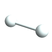
And we can stick the atoms in an Atomset container:

hydrogen = CreateAtomset[{H1, H2}];
hydrogen // ChemView

(*Out:*)

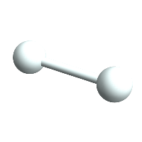
And the fun thing about the mutability here is we can mutate this molecule, but have it be the same thing:

hydrogen // InputForm;
ChemAnimate[
  hydrogen (*object*),
  ChemRotate[2 \[Pi]/36] (*action*),
  36 (*steps*),
  "ChemViewOptions" ->
    {
      ViewPoint -> {0, 0, 5},
      SphericalRegion -> True,
      ImageSize -> 200
      }
  ]

(*Out:*)

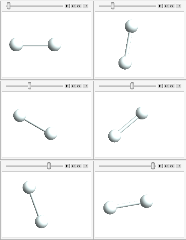
The hydrogen is rotating, no doubt. But it’s always the exact same object, which lets us mutate it with ChemRotate without losing the object. As a further illustration we’ll just move the thing and see that its core data changes, but the object remains the same:

hydrogen0 = hydrogen;
ChemGet[ChemGet[hydrogen, "Atoms"], "Position"]
AtomsetMove[hydrogen, {0, 0, 1}]
ChemGet[ChemGet[hydrogen, "Atoms"], "Position"]
hydrogen0 === hydrogen

(*Out:*)

{ {0, 0, 0}, {1, 0, 0}}

(*Out:*)

{ {0, 0, 1}, {1, 0, 1}}

(*Out:*)

True

So the positions change, but the object remains the same. And we can see why:

hydrogen // InputForm

(*Out:*)

ChemObject["System-default-dd404642-ef6b-4981-9313-a884bff5bce8", 
 "Atomset-6-7fa0bcf3-ea91-46bd-a844-c8b65833daba"]

All it is is a pointer. And we can look at the core data:

$ChemicalSystems[
  "System-default-dd404642-ef6b-4981-9313-a884bff5bce8",
  "Atomset-6-7fa0bcf3-ea91-46bd-a844-c8b65833daba"
  ]

(*Out:*)

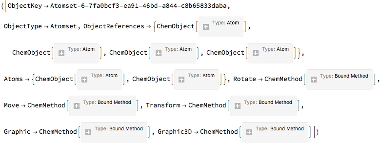
And as planned, the object is just a glorified Association . Except, again, as planned, everything is vectorized. Consider the way we got our atom positions. It was a vectorized call. And we can set in a threaded, vectorized manner, too:

ChemThreadSet[
   ChemGet[hydrogen, "Atoms"],
   "Position",
   { {0, 0, 0}, {1, 0, 0}}
   ];
ChemGet[ChemGet[hydrogen, "Atoms"], "Position"]

(*Out:*)

{ {0, 0, 0}, {1, 0, 0}}

And here’s the benefit of this. Let’s make 1000 fluorine atoms and permute their positions randomly:

AbsoluteTiming[
  fluorines = 
    CreateAtom[
     Thread[{"F", RandomReal[{-10, 10}, {1000, 3}]}]];] // First

(*Out:*)

0.616614

timeVec =
  RepeatedTiming[
   ChemThreadSet[fluorines, "Position", 
    RandomReal[{-10, 10}, {1000, 3}]]] // First

(*Out:*)

0.0096

Doing that one-by-one:

timeMap =
  RepeatedTiming[
     MapThread[
       ChemSet[#, "Position", #2] &,
       {
         fluorines,
         RandomReal[{-10, 10}, {1000, 3}]
         }
       ]] // First

(*Out:*)

0.017

timeMap/timeVec

(*Out:*)

1.8

That’s a speed-up of almost 100%. Of course, it’s not always possible to permute positions all at once, but there are many problems whose implementations can be rewritten in such a way.

Pretend Chemistry with Pretend Potentials

One definite pleasure of working with Mathematica is the sheer volume of things it exposes natively. On that front we have not only a native link to PubChem but also some nice pseudo-compilation and some attractive plotting over surfaces .

Which means we can do cool stuff like easily import a molecule from PubChem:

ChemImport[methyloxirane];
ChemView[methyloxirane]

(*Out:*)

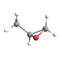
But we can then also compile a function that plots its potential according to its Gasteiger charges :

AtomsetElectricPotential[methyloxirane]

(*Out:*)

And then plot that over its van der Waals surface:

AtomsetElectricPotentialMap[methyloxirane]

(*Out:*)

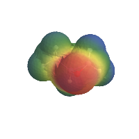
And while there are obviously some sticky implementation details involved in, say, computing the Gasteiger charges, most everything involved in this can be done in fewer than 5 lines of code, which makes the life of the pretend chemist a lot easier.

Pretend Chemistry meets Pretend Data-science

But really that’s just a starting point for pretend science. We can do things one better by doing things like statistical surveys over whole classes of compounds. Maybe we’ll start with pulling in all our alkanes and their PubChem IDs (so we can sort out the ones without IDs):

alkanes = EntityList@EntityClass["Chemical", "Alkanes"];
alkids = ChemDataLookup[alkanes, "PubChemIDs"];
idalks = Pick[alkanes, MatchQ[_Integer] /@ alkids];
idalks~Take~5 // Map[CommonName]

(*Out:*)

{"2,2,4,6,6-pentamethylheptane", "dodecylcyclohexane", \
"trans-p-menthane", "spiropentane", "1,1-dimethylcyclopentane"}

So for most of these things we should be able to get a good 3D structure:

alkobs = DeleteCases[ChemImport@idalks, $Failed];

And we’ll upload these to the cloud for later access (the AtomsetWrapper is a code-as-data wrapper that copies in the atomset data):

alkcache = alkobs // Map[AtomsetWrapper];
CloudExport[alkcache, "MX", "alkane_object_uploads.mx", 
 Permissions -> "Public"]

(*Out:*)

CloudObject["https://www.wolframcloud.com/objects/user-affd7b1c-ecb6-\
4ccc-8cc4-4d107e2bf04a/alkane_object_uploads.mx"]

If you want to import these for your own use (beware – this remains unvectorized and so is slow):

alkobs =
   Map[
     CreateAtomset,
     CloudImport@
       "https://www.wolframcloud.com/objects/b3m2a1/alkane_object_\
uploads.mx"
     ];

Now let’s just look at some simple statistics

alkobs // Length (* Number of molecules *)

alkatels = 
  ChemGet[ChemGet[alkobs, "Atoms"], 
   "Element"]; (* Atom types *)
alkatels // 
 Floor@*Mean@*Map[Length] (* Mean number of atoms *)
alkatels // 
 Floor@*Mean@*
  Map[Length@*Cases["C"]] (* Mean number of carbons *)
alkatels // 
 Floor@*Mean@*Map[Length@*Cases["H"]] (* Mean number of hydrogens *)

(*Out:*)

333

(*Out:*)

30

(*Out:*)

10

(*Out:*)

20

Which gives us a sense for what we’re working with. From this we know our mean degree of unsaturation will be:

degUnsat[c_Integer, h_Integer] :=
   (2 c + 2 - h)/2;
degUnsat[m_List] :=
   
  degUnsat[Length@Cases[m, "C"], Length@Cases[m, "H"]];
degUnsat[10, 20]

(*Out:*)

1

Which is weird, because we explicitly asked for alkanes, but ah well. I guess we’re just workign with hydrocarbons now. In any case, that means most of these things have either a double bond or a ring. Let’s just look at the spread of that:

degsUn = degUnsat /@ alkatels;
Histogram[degsUn]

(*Out:*)

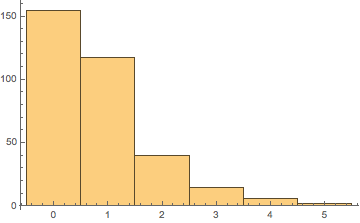
So really most of our sample is saturated alkanes and the small number of highly unsaturated hydrocarbons brings it down to the a DoU of 1.

And just for interest sake we’ll look at those 2 cases where the DoU is 5:

(*Out:*)

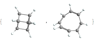
And they’re both rather exotic species. The former being an interesting compound called cubane and the latter being cyclooctatetranene a classic example of *anti* -aromaticity. Both of which have the chemical formula C8H8.

Now as a final example of basic statistics we’ll look at mean bond lengths:

alkbls = AtomsetMeanBondLengths[#, "Type"] & /@ alkobs;

Merge[alkbls, Mean]
Merge[Pick[alkbls, 
  degUnsat[#] == 0 & /@ alkatels], Mean] (* DoU = 0 *)
Merge[
 Pick[alkbls, 
  degUnsat[#] == 1 & /@ alkatels], Mean] (* DoU = 1 *)
Merge[
 Pick[alkbls, 
  degUnsat[#] == 2 & /@ alkatels], Mean] (* DoU = 2 *)
Merge[
 Pick[alkbls, 
  degUnsat[#] >= 3 & /@ alkatels], Mean] (* DoU \[GreaterEqual] 3 *)

(*Out:*)

<|{"C", "C", 1} -> 1.53156, {"H", "C", 1} -> 1.09534, {"C", "S", 1} ->
   1.82033, {"H", "S", 1} -> 1.34111, {"C", "C", 2} -> 
  1.33938, {"C", "Br", 1} -> 1.87237, {"C", "O", 1} -> 
  1.4219, {"H", "O", 1} -> 0.972688|>

(*Out:*)

<|{"C", "C", 1} -> 1.53617, {"H", "C", 1} -> 1.09552, {"C", "S", 1} ->
   1.82033, {"H", "S", 1} -> 1.34111|>

(*Out:*)

<|{"C", "C", 1} -> 1.52729, {"H", "C", 1} -> 1.09552|>

(*Out:*)

<|{"C", "C", 1} -> 1.52987, {"H", "C", 1} -> 1.09534|>

(*Out:*)

<|{"C", "C", 1} -> 1.52671, {"H", "C", 1} -> 1.09336, {"C", "C", 2} ->
   1.33931|>

So somehow our data is doubly weird. Not only is it not all alkanes, it’s not even all hydrocarbons:

Pick[alkobs, MemberQ[Except["H" | "C"]] /@ alkatels] // Length
Pick[alkobs, MemberQ[Except["H" | "C"]] /@ alkatels]~Take~5 // 
 Map[ChemView]

(*Out:*)

13

(*Out:*)

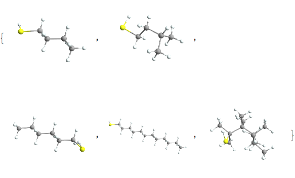
and we would look at that more if we weren’t doing pretend chemistry. But there are some other interesting things here to look at. For instance, our sample contains nothing with a triple bond, which is interesting, but a good thing in what was supposed to be alkanes.

On the other hand, it’s cool to see that the single and double bond lengths gleaned from this match with the expected values quite well, so that is some confirmation for what we did.

Pretend Potentials and Pretend Data-science

With that nice and played with, let’s move on to an even bigger joke. We’ll look at the Gasteiger electric potentials for straight alkane chains.

So first off, we need to find the 320 of our alkobs that are actually hydrocarbons. Then we’ll get the graphs of their carbon atoms so we can look at the branching:

hydobs = Pick[alkobs, FreeQ["S" | "Br" | "O"] /@ alkatels];
hydatels = Select[alkatels, FreeQ["S" | "Br" | "O"]];
hydgraphs = 
  AtomGraph@
     ChemSelect[ChemGet[#, "Atoms"], "Element", MatchQ["C"]] & /@ 
   hydobs;
hydgraphs~Take~3

(*Out:*)

And all three of these clearly need to be dropped, because they branch. We can compute that by figuring out the max chain length and comparing it to the number of nodes:

straighthydobs =
   Pick[hydobs,
     Max[Flatten@#] === Length[#] - 1 &@*GraphDistanceMatrix /@ 
    hydgraphs
     ];
straighthydobs~Take~5 // Map[ChemView]

(*Out:*)

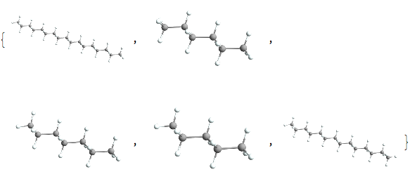
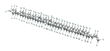
And unfortunately we do only have like 17 of these, but that’s okay. Having so few may even be helpful. We’ll now reorient all of them so they align with one another:

AtomsetAxisAlign[#, "A" -> "X"] & /@ straighthydobs;
straighthydobs // ChemView

(*Out:*)

And now just for fun we’ll calculate their sum electric potential:

pots = AtomsetElectricPotential /@ straighthydobs;
pot =
  With[{pots = pots},
    Compile[{ {p, _Real, 1}},
      Total[Through[pots[p]]]
      ]
    ]

(*Out:*)

And we can plot it, just a standard DensityPlot3D :

straightbounds = {-2, 2} + MinMax@Flatten@# & /@ 
   Transpose[AtomsetBounds /@ straighthydobs];
DensityPlot3D[pot[{x, y, z}],
  Evaluate@Prepend[straightbounds[[1]], x],
  Evaluate@Prepend[straightbounds[[2]], y],
  Evaluate@Prepend[straightbounds[[3]], z]
  ]

(*Out:*)

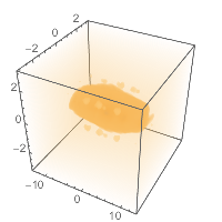
Which gives pretty much what we’d expect, a blobby caterpillar, growing towards the middle.

We can obviously do lots more pretend chemistry, but that suffices, I think, for now, as a good sample of what a nice mixture of OOP and Mathematica can do.